# Library needed to deal with DataFrames
import pandas as pdInteractive, Informative Maps of the Automated Meteorological Data Acquisition System (AMeDAS) Weather Stations in Japan
(A) Data Collection
(B) Data Preprocessing
(D) Data Visualization
weather data
geospatial data
Japan Meteorological Agency
data scraping
data parsing
library - requests
library - bs4
library - pandas
library - re
library - time
library - json
library - jaconv
library - pathlib
Abstract
Searching for the URL of a specific weather station when data scraping from the Japan Meteorological Agency (JMA) website can be time consuming. Especially when the target coordinates are close to a prefectural border, the interface provided on the JMA website is often inadequate. In this project, I present an interactive, informative map that helps data scrapers to quickly locate the target weather station and the parameters needed to designate its URL. The map displays information of the Automated Meteorological Data Acquisition System (AMeDAS) weather stations which was downloaded as a CSV file from the JMA website, combined with the URL information scraped from links on the JMA’s map interface. The data was preprocessed by romanizing the Japanese station names and converting the Japanese calendar to a Gregorian calendar. The data were plotted as an interactive map using Python’s folium library. The resulting project dashboard provides two maps. The smaller map of Japan shows all 1316 weather stations colour-coded to its appropriate jurisdiction. The larger map displays one jurisdictional map in each tab. By clicking a weather station on the jurisdictional map, an informative pop-ups is displayed. The pop-up provides additional information including a small table summarizing the type of weather data recorded at the station, the date that data collection began, the coordinates and elevation of the site, and the height of the thermometer and anemometer. The map helps data scrapers by providing a quick and easy way of accessing the information needed to designate the JMA station URL.
Warning
This project is still ongoing. Documentation is incomplete.
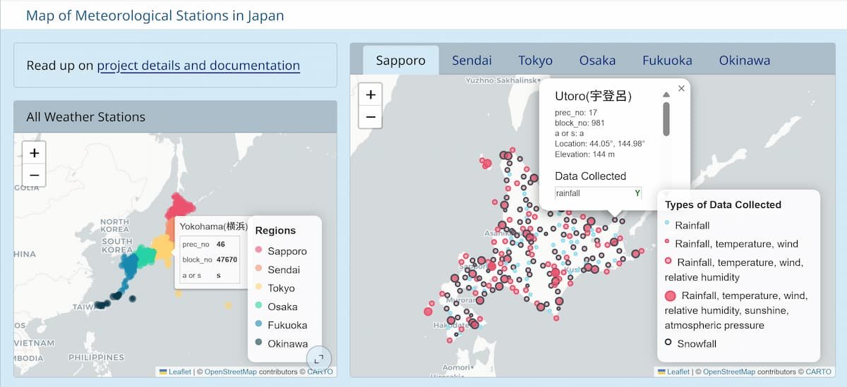
Snapshot of the interactive and informative maps of all AMeDAS weather stations from the Japan Meteorological Agency. Click here to see the maps in action!
1 Updates
2 Skills Demonstrated
A quick run down of the skills I used in this project:
- HTTP requests
- HTML parsing
- regular-expression extraction
- encoding detection
- data cleaning and transformation
- transliteration
- date conversion
- JSON and CSV handling
- file existence checking
- interactive visualization
- HTML generation
3 Introduction
Japan has an extensive weather data collection network, built by the Japan Meteorological Agency (JMA). The foundation for their network is the automatic collection and recording of various weather data at fixed time intervals, called the Automated Meteorologcial Data Acquisition System (AMeDAS). The system started its operation in 1974, and the most basic AMeDAS stations record just rainfall, but are placed at an average interval of 17 km all over Japan1. Fifty years later, as of July 2026, there are a total of 1316 AMeDAS stations in Japan, some of which record rainfall, wind direction and speed, temperature, relative humidity and even snowfall1.
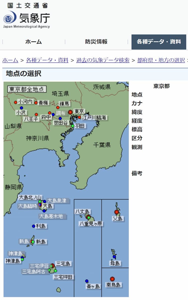
While the comprehensive data collection network provides an abundance of weather data with high geographical precision, finding the weather station closest to a desired location can be a bit tricky. Especially when the target coordinates are close to a prefectural border, the interface on the JMA website is often inadequate, as it cannot show weather stations from multiple neighbouring prefectures (Figure 1).
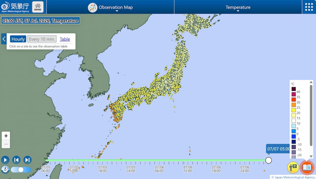
On the other hand, JMA’s AMeDAS observation map, shown in Figure 2, displays all weather stations in one map. The map provides quick access to recent weather data, but it is not useful for data scraping purposes, as it does not provide the URL for accessing past meteorological records.
In this project, I present an interactive, informative map that helps data scrapers to quickly locate the target weather station and the parameters needed to designate its URL. The maps inform the user of the location of the weather station, the station identifiers that constitute parts of the URL, the type of meteorological data that are available from the site, and when data collection of these data began. All data used in this project were available from the JMA website, either as downloadable CSV files or directly scraped from their web source code. As the CSV file is designed with a Japanese reader in mind, I preprocessed the table to make an English user-friendly version and saved the resulting pandas DataFrame. Namely, Japanese station names were converted into romaji (ie. using the English alphabet), and the Japanese calendar dates were changed to a Gregorian calendar. The folium library was used to draw the interactive maps, and a matching legend was generated with the branca library, providing a quick and easy way of accessing the information needed to designate the JMA station URL.
4 Requirements
I have provided all code involved in this project in my GitHub repository. The most informative file is a copy of this web page, available as the map-japan-weather-stations-deets-n-docs.ipynb Jupyter notebook, which explains the steps taken from start to finish of the project. Readers not interested in the data collection and preprocessing may go straight to map generation with the map-japan-weather-stations-dashboard.ipynb Jupyter notebook, or skip ahead to the later sections of the map-japan-weather-stations-deets-n-docs.ipynb notebook.
All files, including the intermediate CSV file containing the preprocessed data, is provided in the data/ subdirectory.
Here is a list of things you’ll need to follow along with how I made the maps.
4.1 Requirements for Running Project From Start to Finish
- A copy of either the
map-japan-weather-stations-deets-n-docs.ipynbJupyter notebook ormap-japan-weather-stations-data-collection-preprocessing.pyPython script from my GitHub repository - A copy of
map-japan-weather-stations-dashboard.ipynbJupyter notebook from my GitHub repository data/subfolder for saving and loading CSV files- Python libraries
requestsbs4pandasretimejsonpathlibjaconvfolium- If
foliummaps do not render in your IDE, you’ll want the following libraries as well:base64IPython
- If you’d like to publish the maps in a Quarto dashboard (as I have done), you will also need Quarto
4.2 Requirements for Just Data Visualization with Maps
If you’re here just to find out how I made the folium maps and the corresponding branca legends, you can skip the data collection and preprocessing steps. Here are the things you’ll need.
- A copy of
map-japan-weather-stations-dashboard.ipynbJupyter notebook from my GitHub repository data/subfolder containing the following files from my GitHub repositoryamedas-stations-all.csv
- Python libraries
pandasfolium- If
foliummaps do not render in your IDE, you’ll want the following libraries as well:base64IPython
- If you’d like to publish the maps in a Quarto dashboard (as I have done), you will also need Quarto
5 Methods
The general steps involved in this project are as follows:
- Collect required data
- Download tabular data on AMeDAS weather stations as a CSV file from the JMA website and read it as a
pandasDataFrame with proper encoding - Scrape, parse and extract identifiers for each JMA weather station (
prec_no,block_noand whether the weather station is anaorstype), from the JMA website’s map interface
- Download tabular data on AMeDAS weather stations as a CSV file from the JMA website and read it as a
- Preprocess data
- Manually convert the Japanese column headers into English
- Convert latitude and longitude from degrees and minutes to decimals
- Transliterate, or spell out Japanese JMA station names based on their phonetics using the Roman alphabet
- Convert the dates that recordings started from Japanese calendar to the Gregorian calendar
- Note which weather data were recorded at each station
- Associate each station with its corresponding URL identifiers including
prec_no,block_noandurl_station_type - Save the preprocessed data as a CSV file
- Visualize the weather stations on a map
foliummap of all 1316 JMA stations with mouseover information- full map could not handle all 1316 stations with mouseover and popup
- circleMarker was used to further simplify the map
foliummap of each jurisdiction with mouseover and popup informationbrancalegends to explain the scatter plot like circle markers on the map
I’ll describe each step detail, starting with the data collection step.
5.1 Data Collection
I collected two pieces of information, both from the JMA website.
- The first information was a CSV file containing information on all current AMeDAS stations in a table format. The CSV file was easily extracted from a downloadable ZIP file on the JMA website, but required some minor deciphering to open the file with the appropriate encoding.
- The second information was data on the URL identifiers needed to access past weather records of each station. These were scraped from the source code on the JMA map interface, and saved as a JSON file for later access.
5.1.1 Download the Table Summary of All AMeDAS Stations
Information about current and past AMeDAS stations, including its station number, its type, its location and when it started recording, are available as PDF or ZIP files (containing a CSV file) on the Japan Meteorological Agency (JMA) website. I have also provided a copy of the CSV file (ame_master_20260324.csv) under the data/ subdirectory in my GitHub repository.
The last part of the file name, _20260324.csv, indicates that the JMA last updated the CSV file on March 24, 2026, most likely reflecting an addition or change in one or more of its AMeDAS weather stations. Depending on when you are reading this documentation, JMA may have a newer version of the file on their website.
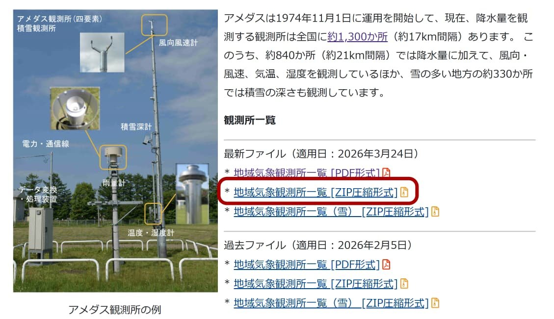
If you would like to check for the latest version of the file, head over to the JMA website, scroll down until you see ‘観測所一覧’ (list of all stations). The latest date that the files were changed are indicated by the date beside ‘最新ファイル’ (newest file). If a newer file than the one I’ve provided is available, you can download the up-to-date file by clicking the second link as shown in red in Figure 3.
Note
For those wondering what the ZIP file in the third link contains, it deals with just the weather stations recording snowfall. As of July 2026, all weather stations recording snowfall also record other meteorological data, making the second ZIP file all inclusive.
TipOpening CSV Files with Unknown Encoding
Downloading and extracting the CSV file ame_master_20260324.csv is quite easy. However, reading the actual data inside the file can be a bit tricky. Specifically, I encountered an UnicodeDecodeError, indicating that the file was not encoded using the commonly used utf-8 paradigm. I needed to pinpoint the encoding model used by the CSV file, and have summarized the steps I took to open a CSV file with unknown encoding in this short blog article.
Once the CSV file was downloaded, I used the pd.read_csv() method from the pandas library to read the CSV file into a DataFrame.
The file encoding for the CSV file was 'CP932', which needs to be specified with the encoding parameter when calling pd.read_csv(). I have summarized the steps involved in opening a CSV file of unknown encoding using charset_normalizer.detect() in a short blog post.
# Read the CSV file as a pandas DataFrame
fileName = './data/ame_master_20260324.csv'
detected_encoding = 'CP932' # Encoding of the CSV file
amedas_df = pd.read_csv(fileName, encoding=detected_encoding)
The .head() method confirms the file has been successfully decoded, and the DataFrame contains the data on the weather stations.
# Check contents of DataFrame
amedas_df.head()| 都府県振興局 | 観測所番号 | 種類 | 観測所名 | カタカナ名 | 気象情報等に表記する名称 | 所在地 | 緯度(度) | 緯度(分) | 経度(度) | 経度(分) | 海面上の高さ(m) | 風速計の高さ(m) | 温度計の高さ(m) | 観測開始年月日 | 備考1 | 備考2 | |
|---|---|---|---|---|---|---|---|---|---|---|---|---|---|---|---|---|---|
| 0 | 宗谷 | 11001 | 四 | 宗谷岬 | ソウヤミサキ | 稚内市宗谷岬 | 稚内市宗谷岬 | 45 | 31.2 | 141 | 56.1 | 26 | 10.1 | 3.1 | 昭53.10.30 | - | - |
| 1 | 宗谷 | 11016 | 官 | 稚内 | ワッカナイ | 稚内市開運 | 稚内市開運 稚内地方気象台 | 45 | 24.9 | 141 | 40.7 | 3 | 24.1 | - | #昭50.4.1 | 11903 | - |
| 2 | 宗谷 | 11046 | 四 | 礼文 | レブン | 礼文町香深 | 礼文郡礼文町大字香深村トンナイ | 45 | 18.3 | 141 | 2.7 | 65 | 9.9 | 3.1 | 平15.10.17 | - | - |
| 3 | 宗谷 | 11061 | 官 | 声問 | コエトイ | 稚内空港 | 稚内市大字声問村字声問 稚内航空気象観測所 | 45 | 24.2 | 141 | 48.1 | 8 | 10 | - | 平15.1.1 | 11904 | 日照・湿度・気圧を除く |
| 4 | 宗谷 | 11076 | 四 | 浜鬼志別 | ハマオニシベツ | 猿払村浜鬼志別 | 宗谷郡猿払村浜鬼志別 | 45 | 20.1 | 142 | 10.2 | 13 | 9.9 | 2.7 | 昭53.10.30 | 11900 | - |
This table contains the majority of the information used to draw out the map, including the latitude and longitude of the weather stations, the name of the weather stations, when data collection began at each site, and the types of the weather stations (which hint at the type of meteorological data collected at the site). However, much of the data is written in Japanese, the dates are noted with Japanese dates (such as 昭53.10.30 or 平15.1.1), and there are certain “exceptions” that need to be considered when scanning for the type of weather data recorded at the station (日照・湿度・気圧を除く means excluding sunshine, relative humidity and atmostpheric pressure).
In other words, the data needs to be cleaned.
However, even before cleaning the data in the DataFrame, I needed to collect one more bit of information. Namely, the bits and pieces of the URL that pinpoint a specific JMA weather station, and are required foraccessing and scraping past weather data.
5.1.2 Data Scraping the prec_no, block_no and JMA station Type from Attributes in the Map Interface HTML
The goal of the interactive map of the weather stations in Japan was to provide a quick and easy method to identify the URL of the weather station closest to some target location. As such, I needed the information on the URL identifiers that gave me access to a specific weather station’s data.
I have documented the full details of crawling the JMA map interface algorithmically to retrieve the URL identifiers for each weather station in this blog post. Below, I’ll briefly go through the steps involved.
Basically, I first identified the three pieces of information that I wanted to extract from each URL (as highlighted in color below):
Wakkanai    data.jma.go.jp/stats/etrn/view/10min_s1.php?prec_no=11&block_no=47401&year=2024&month=3&day=9&view=

Abashiri    data.jma.go.jp/stats/etrn/view/10min_s1.php?prec_no=17&block_no=47409&year=2024&month=3&day=9&view=

Akan        data.jma.go.jp/stats/etrn/view/10min_a1.php?prec_no=19&block_no=0096&year=2024&month=3&day=9&view=

Tokyo       data.jma.go.jp/stats/etrn/view/10min_s1.php?prec_no=44&block_no=47662&year=2024&month=3&day=9&view=

Hakone      data.jma.go.jp/stats/etrn/view/10min_a1.php?prec_no=46&block_no=0390&year=2024&month=3&day=9&view=

Nakatane    data.jma.go.jp/stats/etrn/view/10min_a1.php?prec_no=88&block_no=0897&year=2024&month=3&day=9&view=
Above, I’ve compared the URL of six different weather stations containing meteorological data from March 9, 2024, and highlighted the differences. There are three components of the URL that make it unique to each JMA meteorological station. Namely,
- Whether the JMA station is an
stype oratype (highlighted in red) prec_no(green)block_no(blue)
Thus, I wrote a web crawling algorithm to automatically extract these three pieces of information from the JMA website, and save the results as a nested dictionary in a JSON file named amedas_prec_block_no_dict.json. The overall steps to access the unique identifiers for each weather station were as follows:
- From the starting map interface (Figure 4), scrape all links that lead to a smaller regional map
- Store the complete URLs of each regional map. Crawl one of the regional map URL.
- Scrape all links on the regional map (Figure 5). Each of these links correspond to a weather station.
- Parse the HTML for each weather station and extract the three unique identifiers
- Store the unique identifiers in a nested dictionary
- Repeat for all other weather stations within the regional map (Figure 5)
- Repeat for all other regions within the starting map interface (Figure 4)
- Save the nested dictionary as a JSON file
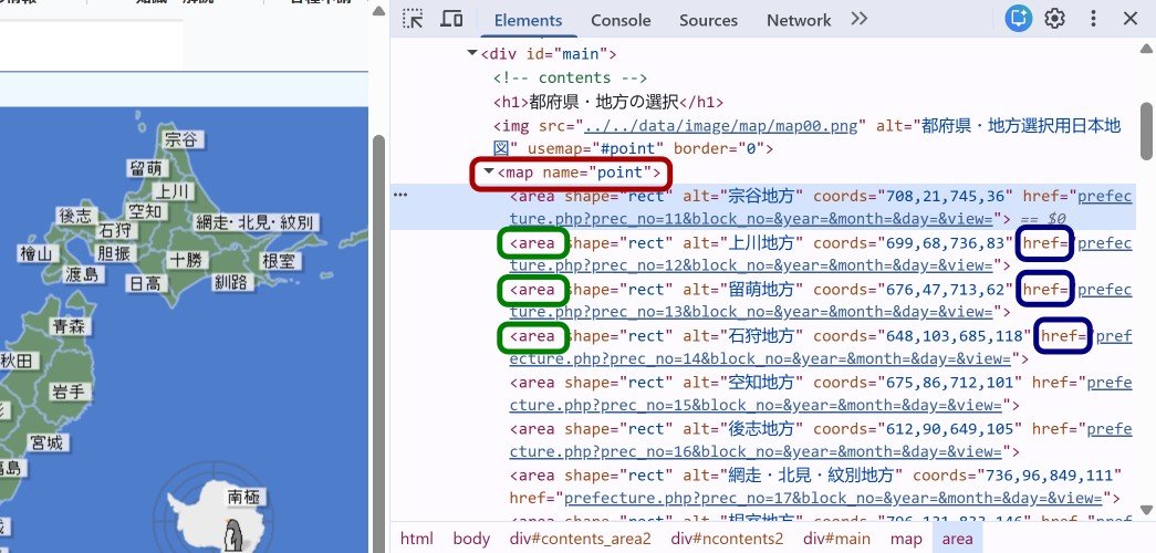
href attribute in the <area> tag, nested within the <map> tag in the starting JMA map interface.
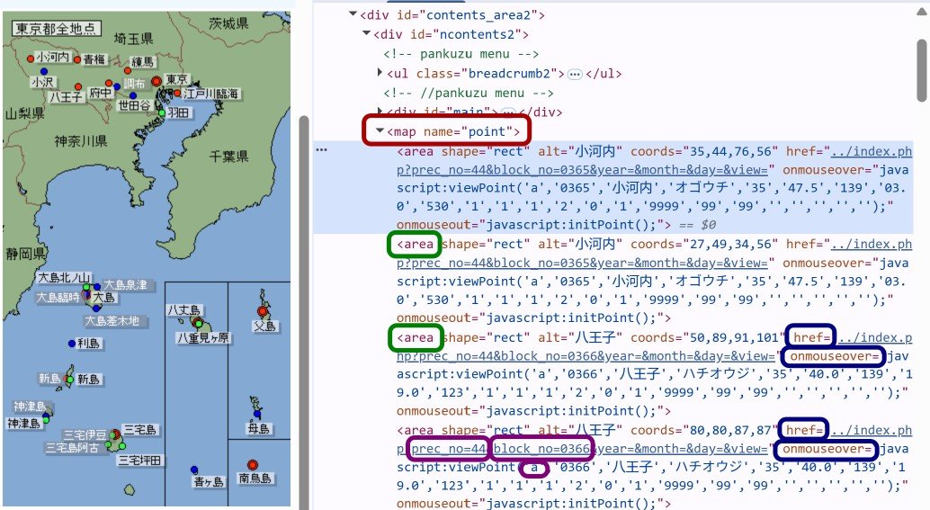
href and onmouseover attributes in the <area> tag, nested within the <map> tag in each JMA regional map interface.
The code below carries out steps 1 and 2 of scraping, parsing and storing the links to the regional map interfaces.
# Import required libraries
import requests
from bs4 import BeautifulSoup
import time
# URL to the starting map interface of Japan
url_japan_map = 'https://www.data.jma.go.jp/stats/etrn/select/prefecture00.php?prec_no=&block_no=&year=&month=&day=&view='
# HTTP request to the starting map
response_japan_map = requests.get(url_japan_map)
# Parse the contents of the Response object (initial HTML parsing)
soup_japan_map = BeautifulSoup(response_japan_map.content, 'html.parser')
# Pause just to make sure we don't rush things
time.sleep(30)
# Take out just the <area> tags, nested within the <map> tag
areas_japan_map = soup_japan_map.find('map').find_all('area')
# Empty list to store all the regional URLs
jma_regional_url_list = []
# Work through the list of area tags to extract the href links
for area_tag in areas_japan_map:
href = area_tag.get('href')
# Add on the base URL to get a full URL
href = 'https://www.data.jma.go.jp/stats/etrn/select/' + href
# Add the full URL to the list
jma_regional_url_list.append(href)Once the URLs for the regional maps are extracted, I went ahead with steps 3 to 8: extracting the three pieces of information needed for pinpointing the URL of each JMA station. I saved the final dictionary as a JSON file called amedas_prec_block_no_dict.json.
# Import additional libraries
from pathlib import Path
import json
# File path to save the final dictionary
fileName = './data/amedas_prec_block_no_dict.json'
# Check if the file exists
#print(f"Python is currently looking here: {Path(fileName).resolve()}")
if Path(fileName).exists():
print("JSON file containing final nested dictionary already exists. \nSkip the algorithmic site crawling process. \nDelete `amedas_prec_block_no_dict.json` file in data subfolder if you would like to run the web crawling process.")
# # Open and load the JSON file containing the dictionary
# with open(fileName, 'r', encoding='utf-8') as file:
# prec_block_as_dict = json.load(file)
else:
print('Starting algorithmic web crawling for URL identifier discovery')
# Final nested dictionary
prec_block_as_dict = {}
# Regular expressions for finding prec_no, block_no and a vs s
re_prec_block = r'prec_no=(\d+)&block_no=(\d+)'
re_a_s = r'javascript:viewPoint\(\'(.)'
# For each regional map URL
for i, url_now in enumerate(jma_regional_url_list):
# Print current region number for every 10th region
if (i + 1) % 10 == 1:
print(f'\tRegion {i+1} out of {len(jma_regional_url_list)}')
# Scrape and initial parsing of the regional map
response = requests.get(url_now)
soup = BeautifulSoup(response.content, 'html.parser')
# Extract the <area> tags for each JMA station nested under the <map> tag
stations_in_region = soup.find('map').find_all('area')
# Use a set to keep track of which weather stations we've entered into the dictionary
duplicate_set = set()
# Work through each weather station inside the region
for station_now in stations_in_region:
# The weather station name (in Japanese) is stored as the `alt` attribute
station_name = station_now.get('alt')
# `href`` attribute for JMA station containing prec_no and block_no and the `onmouseover` containing a vs s
href = station_now.get('href')
onmouseover = station_now.get('onmouseover')
# We can get prec_no and block_no from the href
match_href = re.search(re_prec_block, href)
# If we have no URL match
if match_href == None:
#print('No URL match: ', station_name)
continue
# Prec and block numbers
prec_no = match_href[1]
block_no = match_href[2]
# If we've already added this JMA station (as identified with prec_no and block_no combo), skip
if (prec_no, block_no) in duplicate_set:
continue
else:
# Add to list to prevent duplicate entries for next
duplicate_set.add((prec_no, block_no))
# In case we have no onmouseover attribute
if onmouseover == None:
#print('No onmouseover match: ', station_name)
a_s = 'neither'
else:
# Find the regular expression for a vs s
match_onmouse = re.search(re_a_s, onmouseover)
# Whether the station is a or s
a_s = match_onmouse[1]
# Assign this to a nested dictionary
if station_name in prec_block_as_dict:
# This is when we have a station located elsewhere with the exact same station_name
prec_block_as_dict[station_name].append({'prec_no': prec_no, 'block_no': block_no, 'a or s': a_s})
else:
# For new entries, make a one item list
prec_block_as_dict[station_name] = [{'prec_no': prec_no, 'block_no': block_no, 'a or s': a_s}]
# Sleep between requests
time.sleep(30)
# Write dictionary to a JSON file
with open(fileName, "w", encoding='utf-8') as file:
json.dump(prec_block_as_dict, file, indent=4, ensure_ascii=False) # indent=4 makes it pretty and human-readableJSON file containing final nested dictionary already exists.
Skip the algorithmic site crawling process.
Delete `amedas_prec_block_no_dict.json` file in data subfolder if you would like to run the web crawling process.I set up the code so tha it does not run if the JSON file (containing the nested dictionary) already exists with the if Path(fileName).exists(): statement. This prevents the code from going through the 30 minute algorithmic web crawling loop if it has already done so, and saved its output.
I’ll go ahead and check the contents of the saved dictionary:
# Load the dictionary from the JSON file
with open(fileName, 'r', encoding='utf-8') as file:
    prec_block_as_dict = json.load(file)

# Check some of the dictionary contents
count = 0
for key, value in prec_block_as_dict.items():
    if count % 200 == 0 or key=='大山':
        print(f'station: {key}')
        for list_item in value:
            print(f'\t{list_item}')
    count += 1
station: 稚内
{'prec_no': '11', 'block_no': '47401', 'a or s': 's'}
station: 足寄
{'prec_no': '20', 'block_no': '0109', 'a or s': 'a'}
station: 宮古
{'prec_no': '33', 'block_no': '47585', 'a or s': 's'}
station: 常陸大宮
{'prec_no': '40', 'block_no': '1331', 'a or s': 'a'}
station: 甲府
{'prec_no': '49', 'block_no': '47638', 'a or s': 's'}
station: 大山
{'prec_no': '50', 'block_no': '0446', 'a or s': 'a'}
{'prec_no': '55', 'block_no': '1414', 'a or s': 'a'}
{'prec_no': '69', 'block_no': '0716', 'a or s': 'a'}
station: 松浜
{'prec_no': '54', 'block_no': '1469', 'a or s': 'a'}
station: 津山
{'prec_no': '66', 'block_no': '47756', 'a or s': 's'}
station: 安下庄
{'prec_no': '81', 'block_no': '0779', 'a or s': 'a'}
station: 内之浦
{'prec_no': '88', 'block_no': '0895', 'a or s': 'a'}In the dictionary, the Japanese station name acts as the key, and the value is stored a list of dictionaries. Each nested dictaionry contain the three URL identifiers of prec_no, block_no and a or s. Most station dictionary item contains a list of one item, but some stations, like 大山 or Ooyama station, have multiple stations with identical names.
I have now completed the data collection of this project, gathering the two required information from the JMA website:
- Successfully opened the CSV file containing information on all current AMeDAS stations, and loaded into the workspace as a DataFrame
- Successfully extracted the URL identifiers needed to access each weather station by algorithmically crawling and scraping the HTML of the JMA website, saved the final output as a JSON file, and loaded the output into the workspace as a dictionary
Next is the cleaning or preprocessing of the data.
5.2 Data Preprocessing
The ultimate goal of the data cleaning or preprocessing stage was to generate a pandas DataFrame containing all the data required for drawing the interactive maps. By saving the final DataFrame as a CSV file, I could bypass the data collection and preprocessing step and jump straight into the data visualization step if I ever wanted to change just the look of the maps.
The data collected above were proprocessed as follows:
- Manually convert the Japanese column headers into English
- Convert latitude and longitude from degrees and minutes to decimals
- Transliterate, or spell out Japanese JMA station names based on their phonetics using the Roman alphabet
- Convert the dates that recordings started, from the Japanese calendar to the Gregorian calendar
- Note which data were recorded at each station (eg. rainfall, temperature, relative humidity, etc.)
- Associate each station with its corresponding URL identifiers including
prec_no,block_noandurl_station_type - Save the final preprocessed data as a CSV file
As always, I’ll explain these preprocessing steps in a bit more detail below.
5.2.1 Manually Translate Column Headers
I translated each column header in the existing DataFrame from Japanese and English, and used a dictionary to make the correspondance. The original Japanese column headers were the keys, and its English equivalent were the values. The df.rename() method was used to swap out the column headers.
# Dictionary of Japanese headers to English translations
columns_dict = {'都府県振興局': 'prefectural_bureau',
                '観測所番号': 'station_id',
                '種類': 'station_type',
                '観測所名': 'station_name',
                'カタカナ名': 'katakana_name',
                '気象情報等に表記する名称': 'weather_info_name',
                '所在地': 'location',
                '緯度(度)': 'latitude_degrees',
                '緯度(分)': 'latitude_minutes',
                '経度(度)': 'longitude_degrees',
                '経度(分)': 'longitude_minutes',
                '海面上の高さ(m)': 'elevation',
                '風速計の高さ(m)': 'anemometer_height',
                '温度計の高さ(m)': 'thermometer_height',
                '観測開始年月日': 'observation_start_date',
                '備考1': 'notes1',
                '備考2': 'notes2'}

# Swap out the headers
amedas_df = amedas_df.rename(columns=columns_dict)
Now, the column headers are in English:
# Check the headers in the DataFrame
amedas_df.head(n=1)| prefectural_bureau | station_id | station_type | station_name | katakana_name | weather_info_name | location | latitude_degrees | latitude_minutes | longitude_degrees | longitude_minutes | elevation | anemometer_height | thermometer_height | observation_start_date | notes1 | notes2 | |
|---|---|---|---|---|---|---|---|---|---|---|---|---|---|---|---|---|---|
| 0 | 宗谷 | 11001 | 四 | 宗谷岬 | ソウヤミサキ | 稚内市宗谷岬 | 稚内市宗谷岬 | 45 | 31.2 | 141 | 56.1 | 26 | 10.1 | 3.1 | 昭53.10.30 | - | - |
5.2.2 Convert Latitude and Longitude to Decimals
The original data contained latitude and longitudes as two columns each, separated into degrees (latitude_degrees and longitude_degrees) and minutes (latitude_minutes and longitude_minutes). I simplified this into one decimal notation each.
# Convert degrees and minutes into decimal notation
lat_decimal = amedas_df['latitude_degrees'] + (amedas_df['latitude_minutes'] / 60)
long_decimal = amedas_df['longitude_degrees'] + (amedas_df['longitude_minutes'] / 60)
I then replaced the old latitude and longitude notations in the DataFrame by using the df.insert() method to insert the new columns right next to the existing latitude and longitude columns, and removing the old columns using df.drop().
# Insert the new latitude and longitude right after the existing latitude and longitude
amedas_df.insert(amedas_df.columns.get_loc('latitude_minutes') + 1, 'latitude_decimal', lat_decimal)
amedas_df.insert(amedas_df.columns.get_loc('longitude_minutes') + 1, 'longitude_decimal', long_decimal)

# Remove the old degrees and minutes notation
amedas_df.drop(['latitude_degrees', 'latitude_minutes', 'longitude_degrees', 'longitude_minutes'], axis=1, inplace=True)
The DataFrame now contains a column each for latitude and longitude in decimal notation
# Latitudes and longitudes are now in decimal notation
amedas_df[['station_name', 'latitude_decimal', 'longitude_decimal']].head()| station_name | latitude_decimal | longitude_decimal | |
|---|---|---|---|
| 0 | 宗谷岬 | 45.520000 | 141.935000 |
| 1 | 稚内 | 45.415000 | 141.678333 |
| 2 | 礼文 | 45.305000 | 141.045000 |
| 3 | 声問 | 45.403333 | 141.801667 |
| 4 | 浜鬼志別 | 45.335000 | 142.170000 |
5.2.3 Transliteration of the Japanese Station Names into English
In the DataFrame above, station_name and katakana_name indicate the station names. However both are in Japanese, which is difficult to use for those who are not familiar with the language.
Thus, I used the jaconv library to transliterate, or convert station names from half-width (hankaku) katakana to full-width (zenkaku) katakana, and subsequently to an English alphabet (romaji) name. You can read up on how to use the jaconv and pykakasi, another popular Japanese transliteration library, in this blog post.
For now, I’ll go ahead and transliterate the Japanese station names into English with jaconv.
# Import required libraries
import jaconv
I can use the .apply() method on the DataFrame columns to apply the jaconv.h2z() function to convert from half-width to full-width katakana, and the kata2alphabet() function to transliterate from full-width katakana to the Roman alphabet.
# Convert from half-width to full-width katakana
katakana_full = amedas_df['katakana_name'].apply(jaconv.h2z)

# Convert from full-width to English roman alphabet
romaji_name = katakana_full.apply(jaconv.kata2alphabet)

# Insert the new transliterated name as `romaji_name`
amedas_df.insert(amedas_df.columns.get_loc('katakana_name') + 1, 'romaji_name', romaji_name)
I converted the half-width katakana to full-width katakana before transliterating to English as a direct conversion from half-width katakana to the Roman alphabet encounters issues. This has to do with the differences in the encoding of half-width and full-width katakana letters. I’ve found that converting to full-width katakana, avoids this problem.
The DataFrame now contains a Romanized version of the station name:
# DataFrame has English station names
amedas_df[['station_name', 'katakana_name', 'romaji_name']].head()| station_name | katakana_name | romaji_name | |
|---|---|---|---|
| 0 | 宗谷岬 | ソウヤミサキ | souyamisaki |
| 1 | 稚内 | ワッカナイ | wakkanai |
| 2 | 礼文 | レブン | rebun |
| 3 | 声問 | コエトイ | koetoi |
| 4 | 浜鬼志別 | ハマオニシベツ | hamaonishibetsu |
5.2.4 Convert from Japanese to Gregorian Calendar
In addition to the Japanese alphabet, there is a Japanese calendar.
To be precise, the months and days of the Japanese calendar are the same as the Gregorian calendar, but the naming convention for the year is different. For example, 2026 is considered 令和 (Reiwa) 8th year. Rewind 30 years to 1996: this was the 8th year of the 平成 (Heisei) era. Rewind another 30 years to 1966, and you arrive upon the 41st year of the 昭和 (Shouwa) era.
The Japanese calendar is an era-based system where an old era ends and a new one begins (usually) with the death of the Japanese emperor. I say usually, because the newest 令和 (Reiwa) era actually started with the previous 平成 (Heisei) emperor stepping down from the throne, instead of passing away.
The total number of years in each era is not fixed. The 昭和 (Shouwa) era lasted 64 years, while the 平成 (Heisei) era ended at its 31st year. Some years in the Gregorian calendar are also assigned two eras in the Japanese calendar. For example, the year 1989 is considered both the last year of the 昭和 (Shouwa) era and the first year (also called 元年 (gan-nen)) of the 平成 (Heisei) era. Specifically, January 7th, 1989 is the last day of Showa, and January 8th, 1989 is the first day of Heisei.
While most Japanese people use (and prefer) the Gregorian calendar in their daily lives, many official Japanese documents still use this Japanese calendar. The Japan Meteorological Agency is no exception. As such, the dates that the data collection began for AMeDAS stations is recorded like '昭53.10.30', '平15.10.17', or '令4.11.16', indicating the era, year, month and day.
Feel free to read my blog post on converting Japanese dates into Gregorian dates for more information on the subject. For now, I’ll just briefly explain what I did to convert the Japanese dates into the Gregorian calendar for the purposes of this project.
In the DataFrame we are working with, the observation_start_date are noted as one of four formats:
- The simplest and most intuitive format of
'(One kanji representing the era)(Year number).(Month).(Day)'. All weather data collection at the station began on this date.- Examples:
'昭53.10.30','平15.10.17','令4.11.16'for Shouwa, Heisei and Reiwa, respectively
- Examples:
- Just a
#(not seen in the first 10 entries above), which signifies that data collection began on November 1st, the 49th year of the Shouwa era. This is when the first weather stations began their operation. In other words,#is equivalent to'昭49.11.1'. - A
#, followed by a date in the format of 1. This signifies that precipitation data was first recorded on November 1st, the 49th year of the Shouwa era, but the weather station was later installed with devices to begin data collection on other meteorological parameters.- Example:
'#昭50.4.1'
- Example:
- A combination of two dates with the preceding date in parenthesis. The first date is when rainfall data collection began. All other data recorded at the site began on the second date
- Example:
'(昭50.5.29)昭52.10.24'
- Example:
Due to the complexity of the four scenarios above, I used two different regular expressions to search for # and the Japanese dates written in the format of '(One kanji representing the era)(Year number).(Month).(Day)', and worked through the pandas DataFrame using a for loop instead of carrying out column-wise operations.
I first defined a local function, ConvertJapaneseDates2Gregorian(), which converts a tuple containing the Japanese date in the form of (era, year, month, day) into a string of YYYY-MM-DD corresponding to the Gregorian calendar. The function converts the era based on the following information:
- Showa (昭和) era began on December 25, 1926
- Heisei (平成) era began on January 8, 1989
- Reiwa (令和) era began on May 1, 2019
def ConvertJapaneseDates2Gregorian(str_match):
    """Convert a date in the Japanese calendar to the Gregorian calendar.
    AUTHOR: Mai Tanaka (www.DataDrivenMai.com)
    DATE: 2026-08-13
    REQUIRES: str_match = tuple of the Japanese date in the form (era, year, month, day)
    PROMISES: return_str = string of the date in the Gregorian calendar in the form 'YYYY-MM-DD'
    """

    # Convert year number, month and day from strings into integers
    # Indices 0 and 1 are associated with the year
    era = str_match[0]
    year = str_match[1]

    # If we have '元', convert it to 1
    if year == '元':
        year = 1
    else:
        year = int(year)

    # Indices 2 and 3 are associated with the month and day
    month = int(str_match[2])
    day = int(str_match[3])

    # Convert era names into Gregorian years
    if '昭' in era:
        gregorian_year = year + 1925
    elif '平' in era:
        gregorian_year = year + 1988
    elif '令' in era:
        gregorian_year = year + 2018
    else:
        raise ValueError("Unknown era: {}".format(era))

    # Format the output as yyyy-mm-dd
    return_str = "{}-{:02d}-{:02d}".format(gregorian_year, month, day)
    return return_str
I imported the regex library so that I could search for string patterns in the observation_start_date.
# Import regular expressions library
import re
I worked through the amedas_df DataFrame row-by-row, checking for the four date formats above. I assigned dates to new columns in the DataFrame, 'observation_start_date_rain' and 'observation_start_date_other', according to the four scenarios.
# Two regular expressions
amp_re = r'#'
date_re = r'([昭平令])\.?(元|\d+)\.(\d+)\.(\d+)'

# Make two new columns in the DataFrame
amedas_df.insert(amedas_df.columns.get_loc('observation_start_date') + 1, 'observation_start_date_rain', '')
amedas_df.insert(amedas_df.columns.get_loc('observation_start_date') + 2, 'observation_start_date_other', '')

for i in range(amedas_df.shape[0]):
    # The observation start date
    observation_date = amedas_df.loc[i, 'observation_start_date']

    # Find matches to the two regular expressions
    amp_match = re.search(amp_re, observation_date)
    date_match = re.findall(date_re, observation_date)

    # Temporary storage of the dates
    dates = []

    # Check if we get a match for '#'
    if amp_match:
        dates.append('1974-11-01')

    # Check if we get a match for '([昭平令])\.?(元|\d+)\.(\d+)\.(\d+)'
    if date_match:
        for j in range(len(date_match)):
            # Convert the date to the Gregorian calendar
            new_date = ConvertJapaneseDates2Gregorian(date_match[j])
            dates.append(new_date)

    # Insert the first date we found as rainfall data collection start date
    amedas_df.loc[i, 'observation_start_date_rain'] = dates[0]

    # For all other weather data, the start date for records depends on whether we have a second date or not
    if len(dates) == 2:
        other_date = dates[1]
    else:
        other_date = dates[0]
    amedas_df.loc[i, 'observation_start_date_other'] = other_date
There were two cases I needed to watch out for with the regex searching for '(One kanji representing the era)(Year number).(Month).(Day)' in the observation_start_date.
'元年'instead of'1'for the first year- Typos in data entries
'平.18.3.1'instead of'平18.3.1'
I’ve written a bit more about including exceptions in the regular expressions to accommodate for '元年' (gan-nen) or origin year and dealing with human typos in a previous blog post. You can head on over if you are interested.
For everyone else, you can rest assured that date_re = r'([昭平令])\.?(元|\d+)\.(\d+)\.(\d+)' already works with these exceptions in mind.
The updated DataFrame now has the Gregorian dates for when various meteorological data collection began under the observation_start_date_rain and observation_start_date_other columns.
# Check the DataFrame
amedas_df[['station_name', 'romaji_name', 'observation_start_date', 'observation_start_date_rain', 'observation_start_date_other']].head()| station_name | romaji_name | observation_start_date | observation_start_date_rain | observation_start_date_other | |
|---|---|---|---|---|---|
| 0 | 宗谷岬 | souyamisaki | 昭53.10.30 | 1978-10-30 | 1978-10-30 |
| 1 | 稚内 | wakkanai | #昭50.4.1 | 1974-11-01 | 1975-04-01 |
| 2 | 礼文 | rebun | 平15.10.17 | 2003-10-17 | 2003-10-17 |
| 3 | 声問 | koetoi | 平15.1.1 | 2003-01-01 | 2003-01-01 |
| 4 | 浜鬼志別 | hamaonishibetsu | 昭53.10.30 | 1978-10-30 | 1978-10-30 |
5.2.5 Note Which Weather Data Were Collected at Each Station
One of the requirements of this project was a clear list of the type of meteorological data that were collected and available at each weather station. These could be inferred from a combination of:
- The
station_type'官'types generally recorded all data types, including rainfall, temperature, wind direction and speed, amount of sunshine, relative humidity and atmospheric pressure'三'and'四'type weather stations recorded fewer data'雨'and'雪'type weather stations only recorded rainfall or snowfall, respectively
- Whether
notes1contains another station number- Those with a number also record snowfall
- Exceptions of data types not recorded as noted in
notes2
As with the conversion of Japanese dates to the Gregorian calendar, I worked through the DataFrame row by row to determine the type of weather data collected at each station, and created seven new columns indicating whether a station recorded a specific weather data (Y) or not (N).
The new columns noting whether certain meteorological data were collected were named:
rainfall_YNtemperature_YNwind_YNsunshine_YNrelative_humidity_YNatmospheric_pressure_YNsnowfall_YN
# Work through each row in the DataFrame
for i in range(amedas_df.shape[0]):
    # Pick out the station_type and what the notes say
    station_type = amedas_df.loc[i, 'station_type']
    notes1 = amedas_df.loc[i, 'notes1']
    notes2 = amedas_df.loc[i, 'notes2']

    # YN values to determine. Start with all N
    rainfall_YN = 'N'
    temperature_YN = 'N'
    wind_YN = 'N'
    sunshine_YN = 'N'
    relative_humidity_YN = 'N'
    atmospheric_pressure_YN = 'N'
    snowfall_YN = 'N'

    # Assign the starting YN values according to the station_type
    if (station_type == '官'): # 降水量、気温、風向、風速,日照時間、相対湿度、気圧(一部の観測所を除く)、積雪の深さ(一部の観測所に限る)
        rainfall_YN = 'Y'
        temperature_YN = 'Y'
        wind_YN = 'Y'
        sunshine_YN = 'Y'
        relative_humidity_YN = 'Y'
        atmospheric_pressure_YN = 'Y'
    elif (station_type == '四'): # 降水量、気温、風向、風速、相対湿度(一部の観測所を除く)日照時間の推計
        rainfall_YN = 'Y'
        temperature_YN = 'Y'
        wind_YN = 'Y'
        sunshine_YN = 'Y'
        relative_humidity_YN = 'Y'
    elif (station_type == '三'): # 降水量、気温、風向、風速
        rainfall_YN = 'Y'
        temperature_YN = 'Y'
        wind_YN = 'Y'
    elif (station_type == '雨'):
        rainfall_YN = 'Y'
    elif (station_type == '雪'):
        snowfall_YN = 'Y'

    # If notes1 is not -, it means it also records snowfall
    if notes1 != '-':
        snowfall_YN = 'Y'

    # Note the exceptions of data not recorded in notes2
    if '除く' in notes2:
        if '日照' in notes2:
            sunshine_YN = 'N'
        if '湿度' in notes2:
            relative_humidity_YN = 'N'
        if '気圧' in notes2:
            atmospheric_pressure_YN = 'N'

    # Assign the YN values to the DataFrame
    amedas_df.loc[i, 'rainfall_YN'] = rainfall_YN
    amedas_df.loc[i, 'temperature_YN'] = temperature_YN
    amedas_df.loc[i, 'wind_YN'] = wind_YN
    amedas_df.loc[i, 'sunshine_YN'] = sunshine_YN
    amedas_df.loc[i, 'relative_humidity_YN'] = relative_humidity_YN
    amedas_df.loc[i, 'atmospheric_pressure_YN'] = atmospheric_pressure_YN
    amedas_df.loc[i, 'snowfall_YN'] = snowfall_YN
The DataFrame now clearly notes which weather data are and are not collected at each station.
# The types of weather stations recorded
amedas_df[[
    'station_name',
    'romaji_name',
    'rainfall_YN',
    'temperature_YN',
    'wind_YN',
    'sunshine_YN',
    'relative_humidity_YN',
    'atmospheric_pressure_YN',
'snowfall_YN']].head()| station_name | romaji_name | rainfall_YN | temperature_YN | wind_YN | sunshine_YN | relative_humidity_YN | atmospheric_pressure_YN | snowfall_YN | |
|---|---|---|---|---|---|---|---|---|---|
| 0 | 宗谷岬 | souyamisaki | Y | Y | Y | Y | Y | N | N |
| 1 | 稚内 | wakkanai | Y | Y | Y | Y | Y | Y | Y |
| 2 | 礼文 | rebun | Y | Y | Y | Y | Y | N | N |
| 3 | 声問 | koetoi | Y | Y | Y | N | N | N | Y |
| 4 | 浜鬼志別 | hamaonishibetsu | Y | Y | Y | Y | Y | N | Y |
5.2.6 Assign URL Identifiers for Each Weather Station
As part of the data collection process in Section 5.1.2, I scraped three unique URL identifiers for each weather station and saved it as a JSON file.
# Load the dictionary from the saved JSON file
with open(fileName, 'r', encoding='utf-8') as file:
    prec_block_as_dict = json.load(file)
I incorporated this information into the DataFrame as prec_no, block_no and url_station_type.
Must agree (double check)
If a particular station name, stored in the dictionary as a key, contained a list with one element in it, there was only one weather station with that exact name. For station names where multiple weather stations possessed the same name, I identified the appropriate item from the list, based on its prec_no.
The prec_no saved within the amedas_prec_block_no_dict.json file is associated with the station URL is the information that needed to be assigned to the DataFrame. However, there are two pieces of information contained within the DataFrame, which hint at the prec_no of each weather station:
- The
prefectural_bureau - The first two digits of the
station_id
For example, weather stations in the prefectural_bureau of 宗谷 typical has a station_id starting with 11 (such as 11001 for souyamisaki, or 11176 for toyotomi).
The only caveat is that, these two pieces of information sometimes do not agree with each other, making it difficult to identify a station’s prec_no simply from the information given in the DataFrame (originally extracted from the CSV file downloaded from the JMA website).
As such, when there are multiple stations with the exact same name, I looked at the prefectural_bureau and station_id in the DataFrame, and found an item in the list of weather stations with the same name with a prec_no which agreed with one of the two hints.
To do so, I also needed a dictionary which mapped out the prefectural_bureau with its prec_no. This information was included as part of the amedas_pre_block_no_dict.json file.
I extracted the
# Make a dictionary connecting prefecture name to prec_no
prec_name_no_dict = dict()

# Prefectural bureau names follow one of five patterns
re_prec_name = [r'(.+)地方全地点',
                r'(.+)都全地点',
                r'(.+)府全地点',
                r'(.+)県全地点',
                r'(.+)全地点']

# Work through all items in the dictionary
for station_name, candidate_list in prec_block_as_dict.items():

    # Test if the station_name is actually prefectural_bureau name
    test_match = re.search('全地点', station_name)

    # If we don't get a match, it's just a station name
    if test_match == None:
        continue

    # If we do get a match, find out the exact prefectural_bureau name
    for re_now in re_prec_name:
        prec_match = re.search(re_now, station_name)
        if prec_match:
            match_now = prec_match
            break

    # The prec_name is the first part of the matching regex
    prec_name = match_now[1]

    # Exception is '網走・北見・紋別', which is written as 'オホーツク' in the DataFrame
    if prec_name == '網走・北見・紋別':
        prec_name = 'オホーツク'

    # prec_no is stored in the one-item list
    prec_no = candidate_list[0]['prec_no']

    # Assign prec_no as value into the new dictionary with prefectural_bureau name as key
    prec_name_no_dict[prec_name] = prec_no
I saved the dictionary as a JSON file just in case we’d like to access it later on.
# Save the file as a JSON file just in case
fileName_dict2 = './data/prefectural_bureau_no_dict.json'
with open(fileName_dict2, "w", encoding='utf-8') as file:
    json.dump(prec_name_no_dict, file, indent=4, ensure_ascii=False)  # indent=4 makes it pretty and human-readable

# Load the content of the JSON file to double check
with open(fileName_dict2, "r", encoding='utf-8') as file:
    prec_name_no_dict =  json.load(file)
The dictionary acts as a look up table that attaches a prec_no according to the prefectural_bureau name.
# Take a peek at the first five items in the dictionary
i = 0
for key, value in prec_name_no_dict.items():
    print('prefectural_bureau: ', key, '\tprec_no: ', value)
    i += 1
    if i >= 5:
        break
prefectural_bureau: 宗谷 prec_no: 11
prefectural_bureau: 上川 prec_no: 12
prefectural_bureau: 留萌 prec_no: 13
prefectural_bureau: 石狩 prec_no: 14
prefectural_bureau: 空知 prec_no: 15At first, this seems sufficient to link the station in the DataFrame with the station in the dictionary containing its three URL identifiers. In most cases it is. So, why did I bother looking at the first two digits of the station_id to find out the prec_no that way?
I’ve worked through the 1300+ weather stations, found out the appropriate URL identifiers and assigned them into new columns inside the DataFrame in the code below. I also printed out the stations where the prefectural numbers, identified through the prefectural_bureau and identified through the first two digits of the station_id, do not match.
# Print out simple headers
print('station_name\tpref_bureau\tstation_id\tActual prec_no')

# Make three new columns in the DataFrame
amedas_df.insert(amedas_df.columns.get_loc('station_id') + 1, 'prec_no', '')
amedas_df.insert(amedas_df.columns.get_loc('station_id') + 2, 'block_no', '')
amedas_df.insert(amedas_df.columns.get_loc('station_type') + 1, 'url_station_type', '')

# Work through each row of the DatFrame
for i in range(amedas_df.shape[0]):
    station_name = amedas_df.loc[i, 'station_name']
    block_no = 'Not found' # Initialize block_no to 'Not found'

    # We need to watch out for three station names with alternate names
    if station_name == "つくば":
        station_name = "つくば(館野)"
    elif station_name == "奥日光":
        station_name = "奥日光(日光)"
    elif station_name == "南大東":
        station_name = "南大東(南大東島)"

    # Find the prefectural_bureau, and its corresponding prec_no
    prec_bureau = amedas_df.loc[i, 'prefectural_bureau']
    prec_no1 = prec_name_no_dict[prec_bureau]

    # Find the first two digits in the station_id, which may also be the prec_no
    station_id = str(amedas_df.loc[i, 'station_id'])
    prec_no2 = station_id[0:2]

    # Work through each candidate in the list and find a match
    for list_item in prec_block_as_dict[station_name]:

        # The prec_no of the candidate in the list
        prec_no = list_item['prec_no']

        # One of the prec_no from the DataFrame agree with the candidate in the list
        if prec_no == prec_no1 or prec_no == prec_no2:

            # Find out the block_no and 'a or s'
            block_no = list_item['block_no']
            a_or_s = list_item['a or s']

            # Assign to DataFrame
            amedas_df.loc[i, 'prec_no'] = prec_no
            amedas_df.loc[i, 'block_no'] = block_no
            amedas_df.loc[i, 'url_station_type'] = a_or_s

            # If the prec_no in the DataFrame do not agree, print out some information
            if prec_no1 != prec_no2:
                if station_name == "南大東(南大東島)": # Just to ensure the columns line up
                    station_name = "南大東"
                if prec_no == prec_no2:
                    print(f"{station_name}\t\t{prec_no1}\t\t\033[31m{prec_no2}\t\t{prec_no}\033[0m")
                else:
                    print(f"{station_name}\t\t\033[32m{prec_no1}\033[0m\t\t{prec_no2}\t\t\033[32m{prec_no}\033[0m")

    # If block_no is still as initialized, it means we were unsuccessful in finding a match
    if block_no == 'Not found':
        print('NOT FOUND: ', station_name)
station_name pref_bureau station_id Actual prec_no 幌延 11 13 11 朱鞠内 12 15 12 幌加内 12 15 12 熊石 23 24 23 竜王山 71 72 72 北大東 91 92 91 南大東 91 92 91 旧東 91 92 91 下地島 91 93 91 宮古島 91 93 91 鏡原 91 93 91 城辺 91 93 91 仲筋 91 93 91 伊原間 91 94 91 所野 91 94 91 与那国島 91 94 91 川平 91 94 91 西表島 91 94 91 石垣島 91 94 91 盛山 91 94 91 大原 91 94 91 波照間 91 94 91
There were just over 20 stations, listed above, where the prefectural numbers, as guessed from its prefectural_bureau name and from the starting two digits of the station_id, do not agree with each other. The green numbers indicate instances where the correct prec_no, associated with the actual URL link, agreed with the prefectural_bureau name. However, there was one case where the correct prec_no disagreed with the prefectural_bureau name, and instead, agreed with the first two digits of the station_id, shown in red.
Fortunately, none of these 20+ stations involved those with multiple sites with the same name. However, the code above should be able to deal with such cases, assuming they have substantially different prec_no.
Nonetheless, I generated some robust code to assign the correct prec_no, block_no and the url_station_type into the existing DataFrame.
# Check the prec_no, block_no and url_station_type in the DataFrame
amedas_df[['station_name', 'romaji_name', 'prec_no', 'block_no', 'url_station_type']].head()| station_name | romaji_name | prec_no | block_no | url_station_type | |
|---|---|---|---|---|---|
| 0 | 宗谷岬 | souyamisaki | 11 | 1284 | a |
| 1 | 稚内 | wakkanai | 11 | 47401 | s |
| 2 | 礼文 | rebun | 11 | 1546 | a |
| 3 | 声問 | koetoi | 11 | 1528 | a |
| 4 | 浜鬼志別 | hamaonishibetsu | 11 | 1285 | a |
5.2.7 Saving the Preprocessed Data as a CSV File
The DataFrame, amedas_df was done preprocessing. All the information required for drawing the informative maps were all contained in the DataFrame. Before moving on, I saved the DataFrame as a CSV file using df.to_csv().
# Save the DataFrame as a CSV file
savefileName = './data/amedas_df_all.csv'
amedas_df.to_csv(savefileName, index=False, encoding='utf-8')
Once saved, I could load the DataFrame anytime and anywhere using pd.read_csv(), effectively bypassing the preprocessing step.
# To load the CSV
amedas_df_all = pd.read_csv(savefileName, encoding='utf-8')

# Take a peek inside the loaded DataFrame
amedas_df_all.head()| prefectural_bureau | station_id | prec_no | block_no | station_type | url_station_type | station_name | katakana_name | romaji_name | weather_info_name | ... | observation_start_date_other | notes1 | notes2 | rainfall_YN | temperature_YN | wind_YN | sunshine_YN | relative_humidity_YN | atmospheric_pressure_YN | snowfall_YN | |
|---|---|---|---|---|---|---|---|---|---|---|---|---|---|---|---|---|---|---|---|---|---|
| 0 | 宗谷 | 11001 | 11 | 1284 | 四 | a | 宗谷岬 | ソウヤミサキ | souyamisaki | 稚内市宗谷岬 | ... | 1978-10-30 | - | - | Y | Y | Y | Y | Y | N | N |
| 1 | 宗谷 | 11016 | 11 | 47401 | 官 | s | 稚内 | ワッカナイ | wakkanai | 稚内市開運 | ... | 1975-04-01 | 11903 | - | Y | Y | Y | Y | Y | Y | Y |
| 2 | 宗谷 | 11046 | 11 | 1546 | 四 | a | 礼文 | レブン | rebun | 礼文町香深 | ... | 2003-10-17 | - | - | Y | Y | Y | Y | Y | N | N |
| 3 | 宗谷 | 11061 | 11 | 1528 | 官 | a | 声問 | コエトイ | koetoi | 稚内空港 | ... | 2003-01-01 | 11904 | 日照・湿度・気圧を除く | Y | Y | Y | N | N | N | Y |
| 4 | 宗谷 | 11076 | 11 | 1285 | 四 | a | 浜鬼志別 | ハマオニシベツ | hamaonishibetsu | 猿払村浜鬼志別 | ... | 1978-10-30 | 11900 | - | Y | Y | Y | Y | Y | N | Y |
5 rows × 28 columns
5.3 Data Visualization on folium Maps
My objective of this project was to provide a map that guides programmers scraping data from the Japan Meteorological Agency (JMA) website. I needed a map that displayed:
- The physical location of each weather station on a map of Japan, in the context of all surrounding weather stations (including those that were beyond the prefectural border)
- The URL identifiers of each weather station, needed to pinpoint the URL links to past weather records
- A quick view of types of weather data that were available from each station
After some research, I found the folium library to be best map visualization Python library, suited for my needs. Not only could it plot the stations on a map, it allowed for hover over and pop up text, which I could use to display the URL identifiers and the types of weather data collected at the site.
Experimentation with the folium library revealed some issues that I needed to work through.
- Due to memory constraints with the Jupyter notebook, all 1316 JMA weather stations could not be rendered on one map with
folium.Marker() - The lighter
folium.CircleMarker()method was able to draw all 1316 weather stations, but could not handle information heavy pop up text- The map could handle mouseover text for all 1316 stations
I worked around these issues by opting to draw two maps.
- A small
foliummap of all 1316 JMA stations with mouseover information, displaying- station location
- station name
- URL identifiers
- A larger
foliummap for each of the six jurisdictions with mouseover and pop up text information, displaying- station location
- station name
- URL identifiers
- Types of weather data collected at the station
- Dates that data collection began
Additionally, I added matching branca legends to each map.
Below, I explain how I used folium and branca libraries to draw each map and legend. For step-by-step explanations for plotting scatter plot like circle markers on folium maps or in-depth explanation of using inline and internal CSS and HTML to create custom branca legends, head over to my previous blog posts.
5.3.1 Using an API Key
I registered for CARTO’s free tier to access cartodb voyager map tiles to generate clean looking maps. For obvious security reasons, the free, personal CARTO API key was saved in a separate, invisible .env file, under the variable name of carto_api_key.
I used the dotenv.load_dotenv() function to load the .env file, and the os.getenv() function to retrieve my carto_API_key.
# Load the appropriate libraries
from dotenv import load_dotenv
import os
# Import .env file containing the API key for CARTO ('carto_API_key')
if load_dotenv():
# CARTO API key (request one free at https://carto.com/basemaps/apikey)
carto_api_key = os.getenv('carto_API_key')
# Construct the tile URL template with the API key parameter
tile_url = f"https://basemaps.cartocdn.com/rastertiles/voyager/{{z}}/{{x}}/{{y}}.png?key={carto_api_key}"
# Manual attrition needed
attr = '© <a href="https://www.openstreetmap.org/copyright">OpenStreetMap</a> contributors © <a href="https://carto.com/attributions">CARTO</a>'
else:
# If no .env file, use open street map
tile_url = 'https://tile.openstreetmap.org/{z}/{x}/{y}.png'
# Attrition
attr = '© <a href="https://www.openstreetmap.org/copyright">OpenStreetMap</a> contributors'The else statement above allows me to run the code, even if my .env file was unavailable. If the code cannot find my the file and its API key, I designed it to work with the OpenStreetMap map tile.
5.3.2 Drawing a Small Map with All Weather Stations
I drew the folium maps using the CARTO API key.
# Import libraries for map
import folium
I decided to color the markers for each station according to the jurisdiction it belonged to. I assigned various other attributes to each of the six jurisdictions inside a dictionary.
- The color scheme to use for the markers in each jurisdiction (eg.
'#EF476F') - The
prec_noranges associated with each jurisdiction as tuple (eg.(11, 24)) - The latitude and longitude to set as the center of the map
- Some padding was added on the right side to make space for the legend
# Make a dictionary to be used when styling the jurisdiction maps
juris_info = {
    'Sapporo': ['#EF476F', (11, 24)],
    'Sendai': ['#F78C6B', (31, 36)],
    'Tokyo': ['#FFD166', (40, 57)],
    'Osaka': ['#06D6A0', (60, 74)],
    'Fukuoka': ['#118AB2', (81, 88)],
    'Okinawa': ['#073B4C', (91, 94)],
}

# Work through each jurisdiction to find the best central coordinates to center the map
for key, val in juris_info.items():
    prec_low = val[1][0]
    prec_high = val[1][1]

    # Using only the rows pertaining to one jurisdiction
    boolMask = (amedas_df_all['prec_no'] >= prec_low) & (amedas_df_all['prec_no'] <= prec_high)
    juris_df = amedas_df_all[boolMask].reset_index(drop=True)

    # Max and min of latitude and longitudes
    min_lat = juris_df['latitude_decimal'].min()
    max_lat = juris_df['latitude_decimal'].max()
    min_long = juris_df['longitude_decimal'].min()
    max_long = juris_df['longitude_decimal'].max()

    # Find the center point in latitude, and add some padding on right hand side of longitude
    mid_lat = min_lat + ((max_lat - min_lat) / 2)
    mid_long = min_long + ((max_long - min_long) / 2) + (max_long - min_long) * 0.3

    # Append the location as tuple to the dictionary entry
    juris_info[key].append((mid_lat, mid_long))
I drew a folium.Map() with the following parameters:
location=[mid_lat, mid_long]to center the map on the middle point of all station coordinates, leaving a bit of space for the legend on the right side.zoom_start=3ensured that all of Japan was visible in the windowtiles=tile_urlused thecartodb positronmap style accessed with my personal API keyattr=attrdesignated the attrition or credits for the map tileprefer_canvas=Trueallows me to draw the 1300+ weather stationswidth='100%'andheight='100%'simply allows the map to fill the space available
# Get the central location for the map
min_lat = min(amedas_df_all['latitude_decimal'])
max_lat = max(amedas_df_all['latitude_decimal'])
mid_lat = min_lat + ((max_lat - min_lat) / 2)
min_long = min(amedas_df_all['longitude_decimal'])
max_long = max(amedas_df_all['longitude_decimal'])
mid_long = min_long + ((max_long - min_long) / 2) + ((max_long - min_long) * 0.1) # Bit of padding added for legend

# Generate folium map of Japan
m = folium.Map(
    location=[mid_lat, mid_long],
    zoom_start=3,
    tiles=tile_url,
    attr=attr,
    prefer_canvas=True,
    width='100%',
    height='100%'
    )

# Show map
m
Make this Notebook Trusted to load map: File -> Trust Notebook
I added each station by working through the DataFrame row-by-row, retrieving the prec_no and its corresponding jurisdiction name using PreNo2Name() local function.
def PrecNo2Name(arg_prec_no):
    """Function convert a prefecture number to a jurisdiction name
    AUTHOR:     Mai Tanaka (www.DataDrivenMai.com)
    DATE:       2026-06-30
    REQUIRES:   arg_prec_no = prefectural number (eg. 24)
    RETURNS:    juris_now = name of jurisdiction (eg. 'Sapporo')
    """
    # Simple if-else to get the appropriate jurisdiction
    if arg_prec_no <= 24:
        juris_now = 'Sapporo'
    elif arg_prec_no <= 36:
        juris_now = 'Sendai'
    elif arg_prec_no <= 57:
        juris_now = 'Tokyo'
    elif arg_prec_no <= 74:
        juris_now = 'Osaka'
    elif arg_prec_no <= 88:
        juris_now = 'Fukuoka'
    elif arg_prec_no <= 94:
        juris_now = 'Okinawa'

    return juris_now
I adjusted the marker color according to the jurisdiction, the marker size according to whether the station was a a or s type, and designed the mouseover text to include the URL identifiers available as data in the DataFrame. The markers were created with the designated coordinates, colors, and mouseover text using folium.CircleMarker(), and added to the map using .add_to(m).
# Constants
fill_opacity = 0.6

# Map the JMA stations as circle markers with mouse over information
for rowNow in amedas_df_all.itertuples():

    # From the prefecture number, get the jurisdiction name (and thus its marker color)
    juris_now = PrecNo2Name(rowNow.prec_no)
    color_now = juris_info[juris_now][0]

    # Adjust circle marker radius according to size
    if rowNow.url_station_type == 's':
        radius_now = 5
    else:
        radius_now = 3

    # Make the html to display information when mouse hovers over the circle marker
    mouseover_info = f"""
    <h5>{rowNow.romaji_name.capitalize()}({rowNow.station_name})</h5>
    <table border="1" cellpadding="3">
    <tr><td>prec_no</td> <td><b>{rowNow.prec_no}</b></td></tr>
    <tr><td>block_no</td> <td><b>{rowNow.block_no}</b></td></tr>
    <tr><td>a or s</td> <td><b>{rowNow.url_station_type}</b></td></tr>
    </table>
    """

    # Add the circle marker to the folium map
    markerNow = folium.CircleMarker(
        location=[rowNow.latitude_decimal, rowNow.longitude_decimal],
        tooltip=mouseover_info,
        color=color_now,
        stroke=False,
        fill=True,
        fill_opacity=fill_opacity,
        radius=radius_now
    ).add_to(m)

# Show map
m
Make this Notebook Trusted to load map: File -> Trust Notebook
This generated a map with all 1316 weather stations of Japan, color coordinated according to the six jurisdictions. Each station had mouseover text that displayed the station name as well as its three unique URL identifiers.
5.3.3 Legend for the Small Map of Japan
Once the weather stations were all plotted, I needed a matching legend. This was created with the branca library.
# Import library for legend
import branca
As mentioned before, you can read up on the details of how I created custom branca legends using internal CSS, inline CSS and HTML. Here, I will skip the details and explain the important points.
First of all, folium does not have a built-in method to automatically generate a legend from the items drawn on the map. As indicated in the folium tutorial, legends have to be manually generated using HTML. Basically, the legend HTML is created as a string, and is enclosed within {% macro html(this, kwargs) %}...{% endmacro %}:
legend_html = """
{% macro html(this, kwargs) %}
<div>
    ...HTML generating the legend...
</div>
{% endmacro %}
"""
This legend_html string is fed into a branca.element.MacroElement() object to overwrite the inherited _template. The Python code to do the rewriting looks like this:
legend = branca.element.MacroElement()
legend._template = branca.element.Template(legend_html)
By overwriting the branca.element.MacroElement() object’s template with a custom HTML (and subsequently displaying this macroelement in the map), I can create a map legend. To add the legend to the folium.Map() object, the .add_child(legend) method is used:
m.get_root().add_child(legend)I split up the HTML to feed into the branca.element.Template() into two sections, enclosed in the macros. The two sections in the HTML were:
- An internal CSS containing classes with style and attributes common across multiple elements within the map
- The body HTML dictating the legend structure, containing inline CSS which changed according to user input, and inheriting internal CSS by specifying classes
The basic HTML structure was as follows:
legend_html = """
{% macro html(this, kwargs) %}

<style type='text/css'>
... Common style and attributes assigned to classes ...
</style>

<div
    ... Assign a class to inherit internal CSS for the legend box ...
    ... Assign inline CSS according to user input for the legend box ...
    >
    <div ... Designate internal CSS class for legend title ...> ... Legend Title ... </div>
        <div>
            <ul ... Designate internal CSS class for legend entries ...>
                <li><span
                    ... Assign inline CSS for legend entry ...
                    ></span>
                    ... Description for legend entry ...
                </li>
                ... Repeat for all legend entries ...
            </ul>
        </div>

</div>

{% endmacro %}
"""
Specifically, for the internal CSS, I created classes to inherit the common attributes for:
.map-legendclass.legend-titleclass.legend-labelsclass.legend-labels li spanclass to create circle markers
# Macro start and end, and CSS properties to include as internal CSS enclosed in <style> tags
macro_start = '{% macro html(this, kwargs) %}'
macro_end = '{% endmacro %}'

# Internal CSS common to all legends created in dashboard
legend_css = """
<style type='text/css'>
.map-legend {
    position: fixed;
    z-index: 9999;
    background-color: rgba(255, 255, 255, 0.9);
    box-shadow: 0 0 15px rgba(0, 0, 0, 0.2);
    border-radius: 10px;
    padding: 10px;
    font-family: Arial, sans-serif;
    font-size: 14px;
}
.legend-title {
    font-weight: bold;
    margin-bottom: 8px;
}
.legend-labels {
    list-style-type: none;
    margin-bottom: 5px;
}
.legend-labels li span {
    float: left;
    margin-right: 8px;
    margin-top: 3px;
    border-radius: 50%;
}
</style>
"""
I opted to use a Python dictionary to store the CSS properties and values to use in the creation of the legend. This would allow for the storage of the CSS property like description as a key, as weel as the value to assign to it. I coded a local function, GenerateLegendHTML(), which could take in the dictionary as an argument and integrate the data into the inline CSS, generate a list of legend entries from a nested Python dictionary, and return an appropriate HTML.
def GenerateLegendHTML(dict_legend):
    """Function to generate the HTML for stylized legend boxes with a legend title and circle markers
    AUTHOR:     Mai Tanaka (www.DataDrivenMai.com)
    DATE:       2026-09-08 (edited 2026-09-21 to account for no stroke color)
    REQUIRES: dict_legend = dictionary containing legend id and CSS properties and values including marker visuals in a nested dictionary
    PROMISES: legend_html = string containing HTML and inline CSS for generating stylized legend with markers
    """

    # Check the position of the legend key
    if 'bottom' in dict_legend:
        bottom_pos = dict_legend['bottom']
        top_pos = 'auto'
    elif 'top' in dict_legend:
        top_pos = dict_legend['top']
        bottom_pos = 'auto'
    if 'left' in dict_legend:
        left_pos = dict_legend['left']
        right_pos = 'auto'
    elif 'right' in dict_legend:
        right_pos = dict_legend['right']
        left_pos = 'auto'

    # Add on the new legend HTML legend to the exsiting HTML
    legend_html = f"""
        <div id='{dict_legend['id']}'
            class='map-legend'
            style='
                position: fixed;
                bottom: {bottom_pos};
                top: {top_pos};
                right: {right_pos};
                left: {left_pos};
                width: {dict_legend['box_width']};
                height: {dict_legend['box_height']}
            '>
            <div class='legend-title'>{dict_legend['title']}</div>
            <div>
                <ul class='legend-labels'>
    """
    # Enter the HTML up to the start of the unordered list

    # Create each legend entry
    for entry_now in dict_legend['entries']:

        # Convert the stroke and fill colors from hex to rgb
        rgb_fill = str(ColorHex2RGB(entry_now['marker_fill']))
        rgb_str = str(ColorHex2RGB(entry_now['stroke_color']))

        # Take out the parenthesis and add the alpha or opacity
        fill_rgba = rgb_fill[1:-1] + ', ' + str(entry_now['fill_opacity'])

        # Insert stroke only if opacity is above 0%
        if entry_now['stroke_opacity'] == 0:
            stroke_html = ''
        else:
            stroke_rgba = rgb_str[1:-1] + ', ' + str(entry_now['stroke_opacity'])
            stroke_html = f'border: 2px solid rgba({stroke_rgba});'

        # Make the appropriate HTML for the legend entry
        marker_html = f"""
                    <li><span
                        style='
                            height: {entry_now['marker_height']};
                            width: {entry_now['marker_width']};
                            background: rgba({fill_rgba});
                            {stroke_html}
                        '></span>
                        {entry_now['description']}
                    </li>
        """

        # Add on the marker_html to the legend_html
        legend_html += marker_html

    # Concatenate the closing HTML tags for the unordered list, the <div> containing the unordered list, and the <div> for the legend box
    legend_html += """
                </ul>
            </div>
        </div>
    """

    return legend_html
I also needed a short function ColorHex2RGB() as I had stored the color scheme of the jurisdictions in hexadecimals, but the HTML was using rgba() notation.
def ColorHex2RGB(hex_str):
    """Function to convert the hexadecimal color to RGB notation
    AUTHOR:     Mai Tanaka (www.DataDrivenMai.com)
    DATE:       2026-06-30
    REQUIRES:   hex_str = hexadecimal notation of the color (eg. '#06D6A0')
    RETURNS:    rgb_val = RGB values in a list (eg. [6, 214, 160])
    """
    # Remove the hash symbol
    hex_str = hex_str.lstrip('#')

    # Convert hex pairs to integers
    rgb_val = []
    for i in (0, 2, 4):
        rgb_val.append(int(hex_str[i:i+2], 16))

    return rgb_val
With these functions in place, I could create a custom legend for the map of Japan containing all 1316 JMA weather stations with a legend_dict dictionary containing the CSS properties and values for the legend:
'id'assigns a specific ID to the legend element'title'designates the legend title'top'or'bottom'specifying the location of the legend box from the top or bottom in pixels as a string (eg.'20px')'left'or'right'specifying the location of the legend box from the left or right in pixels as a string (eg.'50px')'box_width''box_height''entries'containing a list of dictionaries to design the legend entries
# Constants
marker_size = '9px'
stroke_opacity = 0

# Make a dictionary for the legend with empty list for the legend entries
legend_dict = {
    'id': 'map-legend-1',
    'title': 'Regions',
    'bottom': '20px',
    'right': '20px',
    'box_width': 'auto',
    'box_height': 'auto',
    'entries': [],
}
Since the entries inside the dictionary above is empty, I needed to populate it with the appropriate information. Each element in this list is a Python dictionary consisting of the following keys:
'description'or text following the circle marker'marker_fill''fill_opacity''stroke_color''stroke_opacity''marker_height'and'marker_width'which designate the marker size
# Make the legend entries as dictionaries and populate the 'entries'
# Loop to make legend entries corresponding to each jurisdiction
for key_juris, value_juris in juris_info.items():
    # Make the dictionary for the marker
    marker_dict = {
        'description': key_juris,
        'marker_fill': value_juris[0],
        'fill_opacity': fill_opacity,
        'stroke_color': value_juris[0],
        'stroke_opacity': stroke_opacity,
        'marker_height': marker_size,
        'marker_width': marker_size,
    }

    # Append this marker dictionary to the legend dictionary
    legend_dict['entries'].append(marker_dict)
Once the dictionary was complete, I generated the HTML for the legend by calling the GenerateLegendHTML() function and added it to the map.
# Create legend_html using the legend_dict and concatenate it all
legend_html = GenerateLegendHTML(legend_dict)
legend_html_all = macro_start + legend_css + legend_html + macro_end

# Create a branca macroelement object and overwrite it with our legend html
legend = branca.element.MacroElement()
legend._template = branca.element.Template(legend_html_all)

# Add the legend to the map
m.get_root().add_child(legend)

# Show map
m
Make this Notebook Trusted to load map: File -> Trust Notebook
Thus, I was able to create a matching legend for the map displaying all 1316 weather stations of Japan.
5.3.4 Drawing a Jurisdictional Map with a Matching Legend
While the small map of Japan was sufficient in displaying
- Weather station location
- Weather station name
- URL identifiers of the station
It was unable to tell me what sort of data was available at each station. While I explain the full details on how I plotted circle markers on folium maps, complete with mouseover and pop up text in a previous blog post, I will explain the basic steps below.
First, I created a local function GenerateHTML4Popup() which could generate the HTML to insert into the popup=folium.Popup() parameter when calling the folium.CircleMarker() method. I designed the pop up to include the following information:
- Station names in English and Japanese
prec_no,block_no, whether the station isaorstype- Station coordinates and elevation
- Types of weather data collected in a table format
- Thermometer and anemometer heights
- When the station started collecting rainfall data, and all other data
def GenerateHTML4Popup(arg_df_row):
    """Function to generate the HTML to insert into a popup in folium
    AUTHOR:     Mai Tanaka (www.DataDrivenMai.com)
    DATE:       2026-06-30
    REQUIRES: arg_df_row = pandas dataframe row as .itertuples()
    PROMISES: html_popup = html format to pass onto folium html input in popups
    """
    # Determine the color of the Y/N fonts for the data collected
    data_YN = [arg_df_row.rainfall_YN,
               arg_df_row.temperature_YN,
               arg_df_row.wind_YN,
               arg_df_row.sunshine_YN,
               arg_df_row.relative_humidity_YN,
               arg_df_row.atmospheric_pressure_YN,
               arg_df_row.snowfall_YN]
    color_YN = []
    for data_YN_now in data_YN:
        if data_YN_now == 'Y':
            color_YN.append('green')
        else:
            color_YN.append('red')

    # Make the html_popup (contains a table of meteorological data collected)
    html_popup = f"""
    <h3> {arg_df_row.romaji_name.capitalize()}({arg_df_row.station_name})</h3>
    prec_no: {arg_df_row.prec_no}
    <br>
    block_no: {arg_df_row.block_no}
    <br>
    a or s: {arg_df_row.url_station_type}
    <br>
    Location: {arg_df_row.latitude_decimal:.2f}°, {arg_df_row.longitude_decimal:.2f}°
    <br>
    Elevation: {arg_df_row.elevation} m
    <br>
    <br>
    <h4>Data Collected</h4>
    <table border="1">
        <tr>
            <td>rainfall</td>
            <td><span style="color: {color_YN[0]}; font-weight: bold;">{data_YN[0]}</span></td>
        </tr>
        <tr>
            <td>temperature</td>
            <td><span style="color: {color_YN[1]}; font-weight: bold;">{data_YN[1]}</span></td>
        </tr>
        <tr>
            <td>wind direction/speed</td>
            <td><span style="color: {color_YN[2]}; font-weight: bold;">{data_YN[2]}</span></td>
        </tr>
        <tr>
            <td>sunshine</td>
            <td><span style="color: {color_YN[3]}; font-weight: bold;">{data_YN[3]}</span></td>
        </tr>
        <tr>
            <td>relative humidity</td>
            <td><span style="color: {color_YN[4]}; font-weight: bold;">{data_YN[4]}</span></td>
        </tr>
        <tr>
            <td>atmospheric pressure</td>
            <td><span style="color: {color_YN[5]}; font-weight: bold;">{data_YN[5]}</span></td>
        </tr>
        <tr>
            <td>snowfall</td>
            <td><span style="color: {color_YN[6]}; font-weight: bold;">{data_YN[6]}</span></td>
        </tr>
    </table>
    <br>
    Thermometer height: {arg_df_row.thermometer_height} m
    <br>
    Anemometer height: {arg_df_row.anemometer_height} m
    <br>
    <br>
    <h4>Observation Start Dates</h4>
    Rain: {arg_df_row.observation_start_date_rain}
    <br>
    Other: {arg_df_row.observation_start_date_other}
    """

    return html_popup
I had coded the previous GenerateLegendHTML() local function so that it would integrate well with the jurisdictional map. I just needed a dictionary containing a list of the legend entries reflecting the circle markers drawn in the jurisdictional map. To generate this dictionary, I created a CreateLegendDict_Jurisdiction() local function, which reflected the color scheme I assigned to the jurisdiction, and the basic circle marker sizing and stroke colors to reflect various types of weather data collected.
def CreateLegendDict_Jurisdiction(color_now, legend_width_px):
    """Function to create and return a dictionary for the legend with the jurisdiction color
    AUTHOR:     Mai Tanaka (www.DataDrivenMai.com)
    DATE:       2026-09-21
    REQUIRES: color_now = Color associated with the jurisdiction (reflected as marker colors)
              legend_width_px = Width of the legend box in pixels as a string (eg. '220px')
    PROMISES: legend_dict = Dictionary containing legend title, size and legend entries
    """

    marker_1_dict = {
        'description': 'Rainfall',
        'marker_fill': '#90E0EF',
        'fill_opacity': 0.5,
        'stroke_color': '#90E0EF',
        'stroke_opacity': 1.0,
        'marker_height': '6px',
        'marker_width': '6px',
    }
    marker_2_dict = {
        'description': 'Rainfall, temperature, wind',
        'marker_fill': color_now,
        'fill_opacity': 0.2,
        'stroke_color': color_now,
        'stroke_opacity': 1.0,
        'marker_height': '6px',
        'marker_width': '6px',
    }
    marker_3_dict = {
        'description': 'Rainfall, temperature, wind, relative humidity',
        'marker_fill': color_now,
        'fill_opacity': 0.4,
        'stroke_color': color_now,
        'stroke_opacity': 1.0,
        'marker_height': '9px',
        'marker_width': '9px',
    }
    marker_4_dict = {
        'description': 'Rainfall, temperature, wind, relative humidity, sunshine, atmospheric pressure',
        'marker_fill': color_now,
        'fill_opacity': 0.8,
        'stroke_color': color_now,
        'stroke_opacity': 1.0,
        'marker_height': '15px',
        'marker_width': '15px',
    }
    marker_5_dict = {
        'description': 'Snowfall',
        'marker_fill': '#FFFFFF',
        'fill_opacity': 0.5,
        'stroke_color': '#495057',
        'stroke_opacity': 1.0,
        'marker_height': '9px',
        'marker_width': '9px',
    }
    # Integrate the dictionaries above into the dictionary that stores the CSS properties of the legend
    legend_dict = {
        'id': 'map-legend',
        'title': 'Types of Data Collected',
        'bottom': '20px',
        'right': '20px',
        'box_width': legend_width_px,
        'box_height': 'auto',
        'entries': [marker_1_dict, marker_2_dict, marker_3_dict, marker_4_dict, marker_5_dict]
        }

    # Return the legend dictionary
    return legend_dict
Finally, I created a local function, MapJurisdiction(), that used all the functions above, GenerateHTML4Popup(), CreateLegendDict_Jurisdiction(), and GenerateLegendHTML(). Given the jurisdiction name, MapJurisdiction() was able to return a folium map object for the jurisdiction, complete with pop ups and a matching legend.
def MapJurisdiction(juris_now, zoom_start):
    """Function to generate the folium map (m) for a given jurisdiction with popups and legend
    AUTHOR:     Mai Tanaka (www.DataDrivenMai.com)
    DATE:       2026-09-21
    REQUIRES: juris_now = name of jurisdiction to map ('Sapporo', 'Sendai', 'Tokyo', 'Osaka', 'Fukuoka', 'Okinawa')
              zoom_now = starting zoom level for the map
    PROMISES: m = folium map object of the Sendai jurisdiction, complete with popups and legend
    """

    # Constants
    legend_width_px = '220px'

    # Pick up the color, the jurisdiction numbers and the mid point latitude and longitude
    color_now = juris_info[juris_now][0]
    prec_low, prec_high = juris_info[juris_now][1]
    mid_lat, mid_long = juris_info[juris_now][2]

    # Generate a folium map
    m = folium.Map(
        location=[mid_lat, mid_long],
        tiles=tile_url,
        zoom_start=zoom_start,
        min_zoom=5,
        attr=attr,
        prefer_canvas=True,
        width='100%',
        height='100%',
    )

    # Using only the rows pertaining to one jurisdiction
    boolMask = (amedas_df_all['prec_no'] >= prec_low) & (amedas_df_all['prec_no'] <= prec_high)
    juris_df = amedas_df_all[boolMask].reset_index(drop=True)

    # Work through each row to plot a circle marker and generate popups
    for rowNow in juris_df.itertuples():
        # Location of the weather station
        lat_now = float(rowNow.latitude_decimal)
        long_now = float(rowNow.longitude_decimal)

        # Make the mouse over information
        mouseover_info = f"<h5>{rowNow.romaji_name.capitalize()} ({rowNow.station_name})</h5>"

        # Make the popup information
        html_popup = GenerateHTML4Popup(rowNow)

        # Adjust size of marker and fill opacity according to station type
        if rowNow.station_type == '雨' or rowNow.station_type == '雪':
            radius_now = 2
            fill_opacity = 0.5
        elif rowNow.station_type == '三':
            radius_now = 2
            fill_opacity = 0.2
        elif rowNow.station_type == '四':
            radius_now = 3
            fill_opacity = 0.4
        elif rowNow.station_type == '官':
            radius_now = 5
            fill_opacity = 0.8

        # Adjust marker fill and stroke colors
        if rowNow.snowfall_YN == 'Y':
            stroke_color = '#495057'
            if rowNow.station_type == '雪':
                fill_color = 'white'
            else:
                fill_color = color_now
        elif rowNow.station_type == '雨':
            fill_color = '#90E0EF'
            stroke_color = '#90E0EF'
        else:
            fill_color = color_now
            stroke_color = color_now

        # Make the marker and add it to the folium map
        markerNow = folium.CircleMarker(
            location=[lat_now, long_now],
            tooltip=mouseover_info,
            popup=folium.Popup(     # Insert pop up text
                html=html_popup,
                max_width=300,
                max_height=150),
            radius=radius_now,
            weight=2,
            color=stroke_color,
            opacity=1.0,
            fill_color=fill_color,
            fill_opacity=fill_opacity,
            ).add_to(m)

    # Create a legend based on the color of the jurisdiction
    legend_dict = CreateLegendDict_Jurisdiction(color_now, legend_width_px)

    # Create legend_html using the legend_dict and concatenate it all
    legend_html = GenerateLegendHTML(legend_dict)
    legend_html_all = macro_start + legend_css + legend_html + macro_end

    # Create a branca macroelement object and overwrite it with our legend html
    legend = branca.element.MacroElement()
    legend._template = branca.element.Template(legend_html_all)

    # Add the legend to the map
    m.get_root().add_child(legend)

    # Return the map
    return m
Now, creationg of the jurisdictional map only required me to enter the jurisdiction name, and the starting zoom value.
# Designate the jurisdiction and starting zoom level
juris_now = 'Sapporo' # 'Sapporo', 'Sendai', 'Tokyo', 'Osaka', 'Fukuoka', 'Okinawa'
zoom_now = 6

# Create folium map
m = MapJurisdiction(juris_now, zoom_now)

# Show map
m
Make this Notebook Trusted to load map: File -> Trust Notebook
With that, I was able to generate the six jurisdictional maps with pop up text displaying the URL identifiers, and explaining the types of weather data collected, complete with a matching legend.
5.3.5 Quarto Dashboard Basics
In created the dashboard displaying the two interactive maps using Quarto dashboards. While you can read up on the details in the official Quarto documentation, I’ll very briefly explain the format I used.
In the Jupyter notebook file, I included a header:
format:
    dashboard:
        orientation: columns
When I rendered the document using quarto, this would generate a dashboard that was split into columns.
Then, insdie the Jupyter notebook, I designated two columns. The first column had a width=40% and contained the link to this documentation page and the small map of Japan containing all 1316 weather stations. The second column used up the remaining width=60%, with each jurisdictional map being assigned to a tab using .tabset. The .no-scrollbar class is a class I used in my external CSS file to remove scrollbars within the dashboard cards. Each jurisdictional map was generated with #| title: at the start of the Jupyter cell, followed by an appropriate call to the MapJurisdiction() local function.
The general format of the Jupyter notebook to generate the dashboard was as follows:
## {width=40%}
### Top Card
Read up on [project details and documentation](deets-n-docs.html)

### Bottom Card
... code to generate the small map of Japan...

## Column {width=60% .tabset .no-scrollbar}

#| title: Sapporo
... code to generate jurisdictional map of Sapporo ...

#| title: Sendai
... code to generate jurisdictional map of Sendai ...

#| title: Tokyo
... code to generate jurisdictional map of Tokyo ...

#| title: Osaka
... code to generate jurisdictional map of Osaka ...

#| title: Fukuoka
... code to generate jurisdictional map of Fukuoka ...

#| title: Okinawa
... code to generate jurisdictional map of Okinawa ...
6 Results and Discussion
The smaller map of Japan shows all 1316 weather stations color-coded to its appropriate jurisdiction. The larger map displays one jurisdictional map in each tab. By clicking a weather station on the jurisdictional map, an informative pop-ups is displayed. The pop-up provides additional information including a small table summarizing the type of weather data recorded at the station, the date that data collection began, the coordinates and elevation of the site, and the height of the thermometer and anemometer.
Measure how long it takes to search out 10 locations on a map.
Two videos (combine into one video later on)
Snapshot of the interactive and informative maps of all AMeDAS weather stations from the Japan Meteorological Agency. Click here to see the maps in action!
6.1 Limitations
- Romanized version of the station names do not always agree with the commonly known name.
- For example, “トウキョウ” is translated as “Toukyou” or “Tokyou”, while its commonly known name is “Tokyo”
- Similarly, “オオサカ” is displayed as “Oosaka” in my map, but is usually written as “Osaka”
- JMA weather stations that only collect a subset of meteorological data, but have the same station name have slightly inaccurate pop-up information
- The data collection equipment of some stations seem to be located at nearby, but different locations.
- For example, the ‘Obihiro’ station in under the Sapporo jurisdiction has one site collecting temperature, rainfall and snowfall, and a nearby site (with the same name but different coordinates) collecting wind and sunshine data
- For such sites, the tabular data of which data is collected at which site is somewhat mixed. In most cases, all data collected at the other site will also be displayed as a ‘Y’ on the table, with the exception for snowfall data.
- In other words, some JMA weather stations are mapped at two coordinates, with slightly inaccurate table data in the pop-ups.
- Weather data that are not recorded, but should be recorded
- 欠測
6.2 Future Directions
- Enter GPS coordinates, or location name and the type of weather data desired
- Automatically list out closest weather stations that provide the data
- Checks whether certain data are actually available, instead of x or \
7 Conclusions
Restate the objective
Summarize what I did and how much performance was improved Impact
Limitations Future work
8 References
1.
Japan Meteorological Agency. 地域気象観測システム(アメダス). 気象庁 (2026).
9 Further Readings
- Getting a
UnicodeDecodeErrorwhen opening a mystery CSV file? Check out this blog post on reading a CSV file with unknown encoding into apandasDataFrame - Are you scraping from a lot of webpages on the same site? Consider automating the URL retrieval process by algorithmically crawling the web site and automatically retrieving the unique identifiers that allow you to designate the URL
- Read this blog post to transcribe or transliterate Japanese words into the Roman alphabet
- Are Japanese dates giving you headaches? Refer to this blog article on how Japanese dates work and how to convert them to Gregorian dates